library(tidyverse)

iris2 <- iris %>% select(Sepal.Length, Sepal.Width, Petal.Length)
iris2 %>% cor %>% corrplot::corrplot()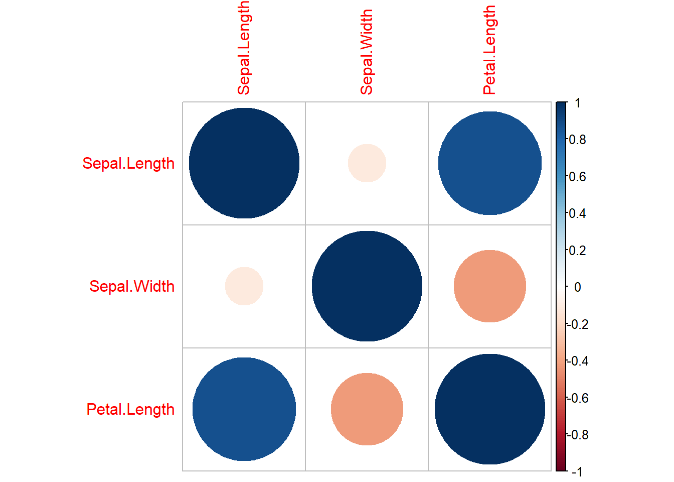
Tree-based models like decision trees, random forest, ligthGBM and xgboost are known, among other qualities, for their robustness to multicollinearity. It’s well known that their predictive power isn’t shaken by the presence of extremely correlated variables.
But who has never used a Random Forest for variable selection? Taking, for example, the top 10 most important ones and dropping the rest?
Or even ventured an interpretation and drew conclusions from the order of the most important variables?
Below we show why we shouldn’t ignore multicollinearity completely!
First let’s fit a nice little model, free of multicollinearity. Suppose we want to predict Petal.Length using the sepal measurements (Sepal.Width and Sepal.Length) from our good old iris dataset.
library(tidyverse)
iris2 <- iris %>% select(Sepal.Length, Sepal.Width, Petal.Length)
iris2 %>% cor %>% corrplot::corrplot()
The plot above shows that the explanatory variables are not strongly correlated. Fitting a random fores, we get the following variable importance order:
library(randomForest)
iris2_rf <- randomForest(Petal.Length ~ ., data = iris2)
varImpPlot(iris2_rf)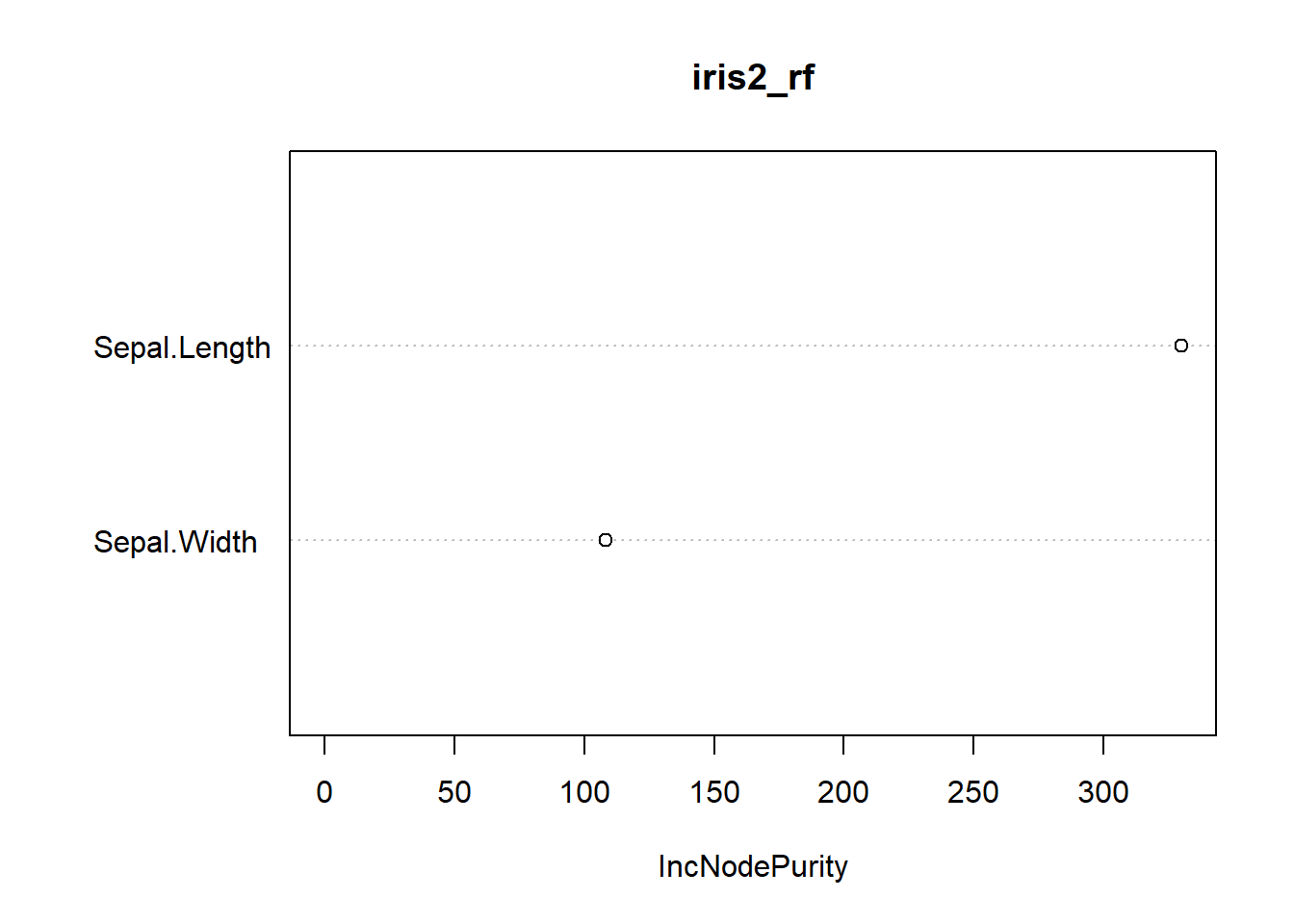
No surprises. Now on to the problem!
Let’s forge an extreme situation where many variables are multicollinear. I’ll do this by repeating the Sepal.Length column several times.
iris3 <- accumulate(1:20, ~{
  .x[[paste0("Sepal.Length", .y)]] <-  iris2$Sepal.Length
  .x
}, .init = iris2)

iris3[[20]] %>% cor %>% corrplot::corrplot(order = "alphabet")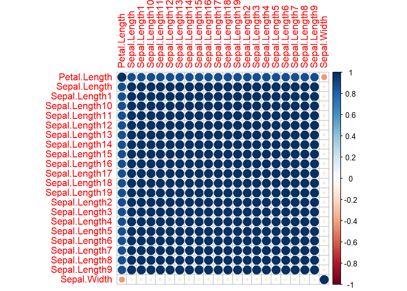
Now things are ugly! We have 20 perfectly collinear variables. Even so, a random forest on this new dataset wouldn’t lose predictive power.
But what happened to the variable importance?
iris3_rf <- randomForest(Petal.Length ~ ., data = iris3[[20]])
varImpPlot(iris3_rf)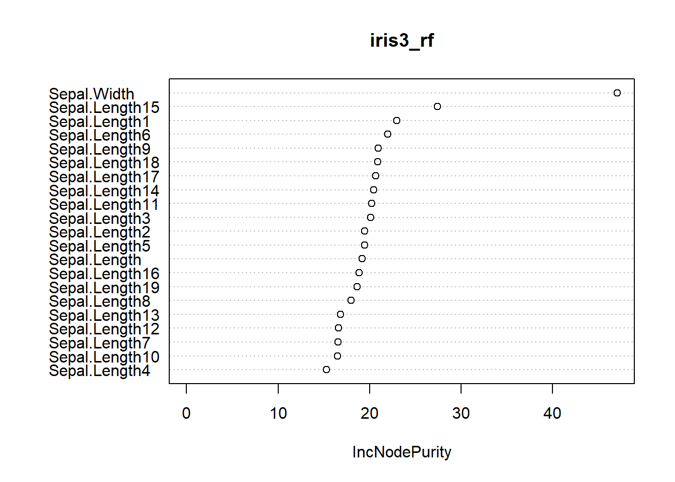
Here the tables have turned: we would conclude that Sepal.Width is the most important of all the variables!
The plot below shows that the more correlated variables we have, the lower the importance of ALL OF THEM AT THE SAME TIME! It’s as if the collinear variables split the importance among themselves.
# fits a random forest on datasets with 1 to 20 repetitions of `Sepal.Length`
rfs <- map(iris3, ~ randomForest(Petal.Length ~ ., data = .x) %>% importance)

# extracts the importances of the `Sepal.Length` repetitions
importancia <- map_dfr(rfs, ~{
  .x %>%
    as.data.frame() %>%
    tibble::rownames_to_column() %>%
    dplyr::filter(stringr::str_detect(rowname, "^Sepal.Length"))
}, .id = "n_repeticoes") %>%
  mutate(n_repeticoes = as.numeric(n_repeticoes))

# Plot of the number of multicollinear variables vs importance
importancia %>%
  ggplot(aes(x = n_repeticoes, y = IncNodePurity)) +
  geom_point() +
  geom_hline(yintercept = 40, size = 1, linetype = "dashed", colour = "red") +
  labs(x = "Qtd de repetições da coluna `Sepal.Length`", y = "Importância", title = "Gráfico da relação entre o número de variáveis multicolineares vs importância")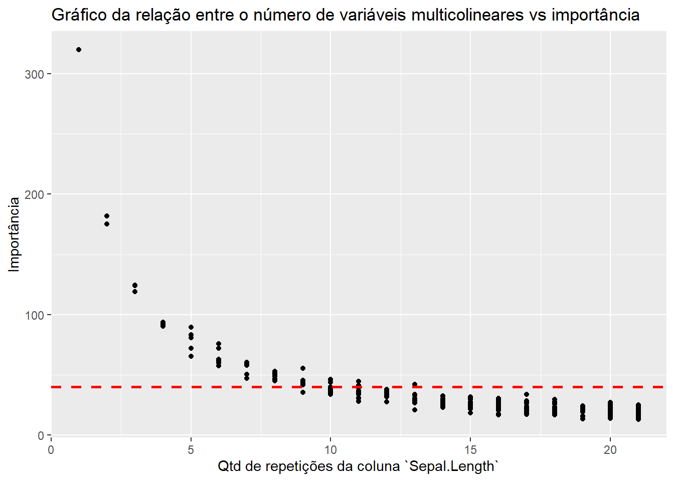
In practice, if we set an importance cutoff to drop variables (as illustrated by the red line), we would have a potential problem: we could be throwing away very important information.
Some ways to deal with multicollinearity are:
Be careful when throwing everything into the pot! We should always worry about multicollinearity, even when fitting tree-based models.
Cheers!