f <- function(x) cos(x*20)
expi <- function(x) cos(x) + sin(x)*1i
L <- 40
medias_Re <- c()
fs <- c()
as <- seq(0.01, 1, l = 140)Winding a cosine around a circle: the Fourier transform in a GIF
concepts
r
fourier transform
animation
An R animation, inspired by 3Blue1Brown, that wraps cos(20t) around the complex plane and tracks its centre of mass as the winding frequency changes.
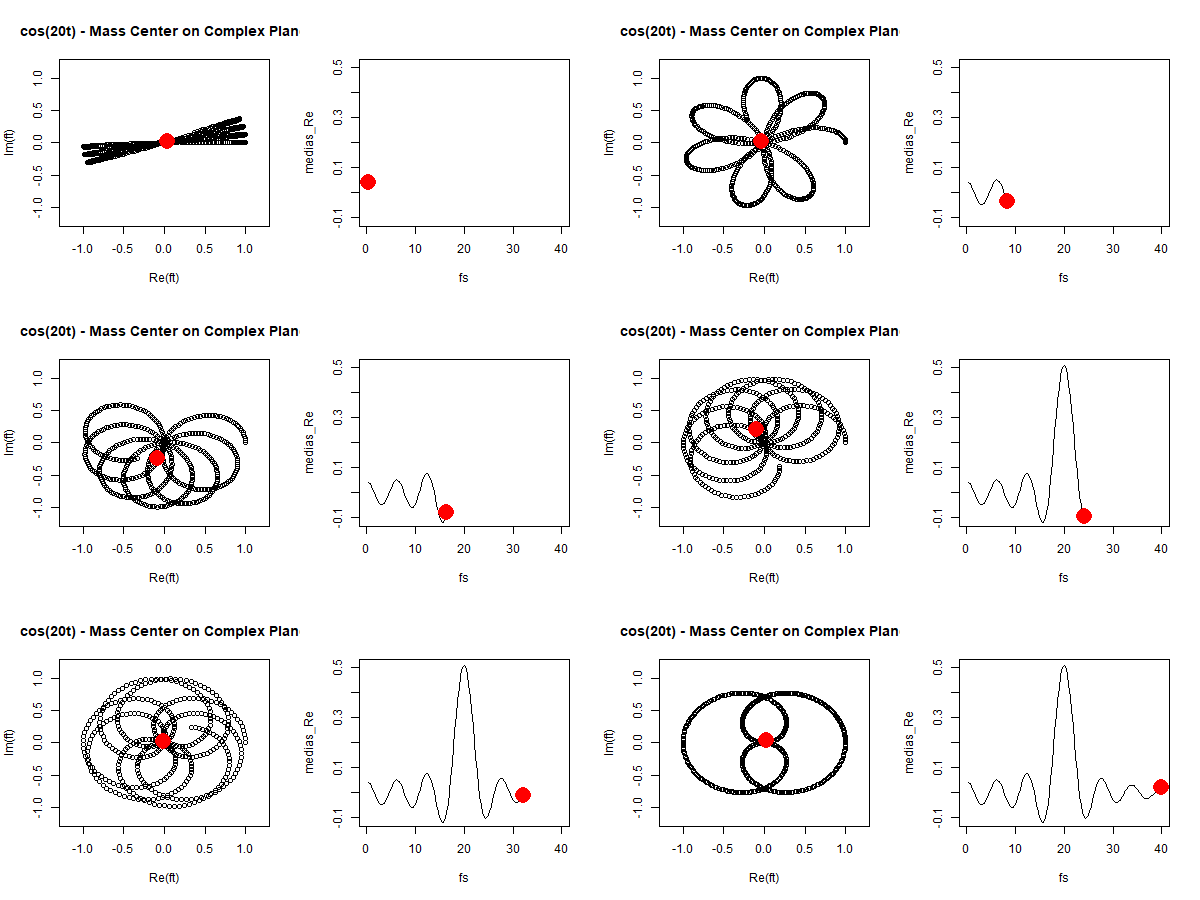
A while ago I posted on LinkedIn an #rstats GIF inspired by 3Blue1Brown’s But what is the Fourier Transform? A visual introduction. This post is that GIF, with the code behind it.
The idea
Take a signal \(g(t)\), here \(g(t) = \cos(20t)\) for \(t\) between 0 and 1, and wrap it around the origin of the complex plane. Each point of the signal becomes \(g(t)\,e^{i\omega t}\): the angle comes from \(t\) and the winding frequency \(\omega\), and the distance from the origin comes from \(g(t)\).
Then take the centre of mass of the wrapped curve, the average of all its points:
\[ \hat{g}(\omega) = \frac{1}{T}\int_0^T g(t)\,e^{i\omega t}\,dt \]
- left panel: the wrapped curve for the current \(\omega\) and its centre of mass (red dot).
- right panel: the real part of the centre of mass as \(\omega\) goes from 0.4 to 40.
For most winding frequencies the curve spreads evenly around the origin and the centre of mass stays near 0. When \(\omega = 20\), the frequency of the cosine, the peaks of the signal all land on the same side of the circle and the centre of mass jumps to about 0.5. That spike is the frequency showing up in the Fourier transform.
The code
f() is the signal and expi() is \(e^{ix}\) written as \(\cos x + i \sin x\). For each a, x runs from 0 to a * L and the signal is evaluated at x / (a * L), which goes from 0 to 1. So expi(x) * f(x / (a * L)) is \(g(t)\,e^{i\omega t}\) with \(\omega = a L\).
The original gist writes the GIF with animation::saveGIF(), which needs ImageMagick, and pauses with Sys.sleep(0.1) between frames. Here gifski::save_gif() records each plot as a frame instead, so par(mfrow = c(1,2)) moves inside the block to apply to the GIF’s device.
gifski::save_gif({
  par(mfrow = c(1,2))
  for(a in as) {
    x <- seq(0, a*40, l = 500)
    ft <- expi(x)*f(x/(a*L))
    media_Re <- mean(Re(ft))
    plot(Re(ft), Im(ft), xlim = c(-1.2, 1.2), ylim = c(-1.2, 1.2), main = "cos(20t) - Mass Center on Complex Plane")
    points(media_Re, mean(Im(ft)), col = "red", cex = 3, pch = 16 )
    medias_Re <- c(medias_Re, media_Re)
    fs <- c(fs, a*L)
    plot(fs, medias_Re, type = "l", xlim = c(0, 40), ylim = c(-0.11, 0.51))
    points(a*L, media_Re, col = "red", cex = 3, pch = 16)
  }
}, gif_file = "fourier.gif", width = 600, height = 300, delay = 0.1)
The video goes further, from this centre-of-mass picture to the Fourier transform formula itself.