library(torch)
torch_manual_seed(1)

x <- torch_tensor(cbind(cars$speed, cars$speed^2))
y <- torch_tensor(cars$dist)$unsqueeze(2)
mse <- nn_mse_loss()

model_gen <- function(lr) {
  lin <- nn_linear(2, 1)  # b0, b1 and b2
  opt <- torch::optim_adam(lin$parameters, lr = lr)
  return(list(lin = lin, opt = opt))
}

model_fit <- function(model) {
  model$opt$zero_grad()

  pred <- model$lin(x) # b0 + b1*speed + b2*speed^2
  custo <- mse(y, pred)
  custo$backward()
  model$opt$step()
  return(pred)
}Gentle introduction to the learning rate parameter
concepts
deep learning
torch
r
optimization
Three copies of the same model, fitted by gradient descent with three different learning rates: too low, too high and just right.
I found an old gist on my GitHub about the learning rate. It fits a regression line by gradient descent, and it’s oddly satisfying to watch. A bit insightful too.
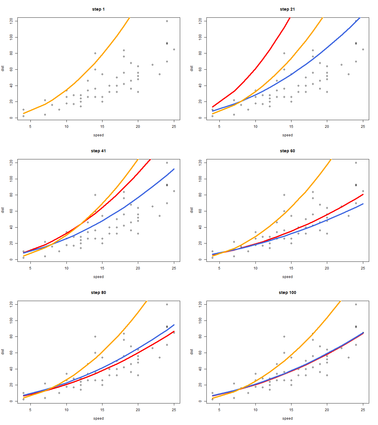
There are three curves, one for each learning rate:
- orange: too low (
lr = 0.001). Each step is tiny, so after 100 steps the curve is still far from the points. - red: too high (
lr = 2). Each step overshoots, so the curve swings far from the points before it settles. - blue: just right (
lr = 0.05). The curve moves steadily toward the points and stays there.
The learning rate
Gradient descent updates the model parameters a little at each step, in the direction that lowers the loss:
\[\theta_{t+1} = \theta_t - \eta \, \nabla L(\theta_t)\]
The learning rate \(\eta\) is the size of that step. The optimizer below is Adam, which adapts the step for each parameter, but the learning rate still sets its scale.
The code
The data is the cars dataset: stopping distance (dist) as a function of speed. The model is dist ~ speed + speed^2, written as a linear layer with two inputs.
Three copies of the same model, one per learning rate:
model1 <- model_gen(2)
model2 <- model_gen(0.05)
model3 <- model_gen(0.001)
Each iteration takes one optimizer step for each model and draws the three fitted curves. The original gist plots to the screen with Sys.sleep(0.1) between steps. Here gifski::save_gif() records each plot as a frame instead.
gifski::save_gif({
  for (i in 1:100) {
    pred1 <- model_fit(model1)
    pred2 <- model_fit(model2)
    pred3 <- model_fit(model3)
    plot(cars, main = paste("step", i))
    lines(x[, 1]$unsqueeze(2), pred1, col = "red", lwd = 4)
    lines(x[, 1]$unsqueeze(2), pred2, col = "royalblue", lwd = 4)
    lines(x[, 1]$unsqueeze(2), pred3, col = "orange", lwd = 4)
  }
}, gif_file = "learning_rate.gif", width = 640, height = 480, delay = 0.1)
Tune your models, folks!